The function map() (maps package), combined with the “worldHires” database from the mapdata package, allows creating a wide variety of geographical maps of world coastlines and national boundaries. The mapdata package contains the full database, approximately 2 million points.
Unfortunately, object returned by the map() function are solely “graphical object” and GIS manipulations and calculations are not possible; for example, values of a raster layer for a specific polygon (e.g. national boundaries) could not be extracted. Moreover, when user is familiar with raster, gdal and sp packages, defining the map projection to use are not simple; which is not achieved by the use of “CRS” of coordinate reference system arguments.
The SpacializedMap() function operates as the map() function, but creates georeferenced map of class SpatialPolygons. User defines the map database and, if needed, the name of the polygon to draw, (i.e. national boundaries, states, islands, etc.). Refer to the map() help page for more details on optional arguments (exact argument can be very usefull). SpatialPolygons thus created, can be transformed to a new coordinate reference system by the use of the spTransform() function (rgdal package).
The SpacializedMap() function helps creating nice figures and maps.
Feel free to use or comment!!
The Function:
SpacializedMap=function(database="world",regions=".",...){
#Create objects of class SpatialPolygons from geographical maps from map() function
#BBORGY 08/20/2014
require(maps)
require(sp)
require(mapdata)
k=map(database=database,regions=regions,plot=F,fill=T,...)
pol=vector("list",length(unique(k$names)))
w.start=c(1,which(is.na(k$x))+1)
w.end=c(which(is.na(k$x))-1,length(k$x));w=1
for(j in 1:length(unique(k$names))){
pol[[j]]=vector("list",sum(k$names==unique(k$names)[j]))
for(i in 1:sum(k$names==unique(k$names)[j])){
pol[[j]][[i]]=Polygon(cbind(k$x[c(w.start[w]:w.end[w],w.start[w])],k$y[c(w.start[w]:w.end[w],w.start[w])]))
w=w+1}
pol[[j]]=Polygons(pol[[j]],unique(k$names)[j])}
pol=SpatialPolygons(pol,proj4string=CRS("+init=epsg:4326"))
return(pol)}
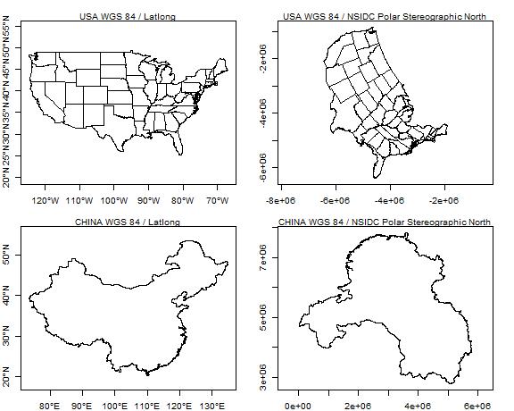
Example 1:
library(rgdal)
par(mfrow=c(2,2),mar=c(2,2,2,2))
pol_WGS84=SpacializedMap('state')
plot(pol_WGS84,axes=T);mtext("USA WGS 84 / Latlong",cex=.8)
pol_NAD87=spTransform(pol_WGS84,CRS("+init=epsg:3413"))
plot(pol_NAD87,axes=T);mtext("USA WGS 84 / NSIDC Polar Stereographic North",cex=.8)
pol_WGS84=SpacializedMap('worldHires','China',exact=T)
plot(pol_WGS84,axes=T);mtext("CHINA WGS 84 / Latlong",cex=.8)
pol_NAD87=spTransform(pol_WGS84,CRS("+init=epsg:3413"))
plot(pol_NAD87,axes=T);mtext("CHINA WGS 84 / NSIDC Polar Stereographic North",cex=.8)
Example 2:
library(raster)
MAT=raster("bio1.bil")
X11(10,5)
par(mar=rep(2.5,4))
image(MAT,main="Mean Annual Temperature",col=rev(heat.colors(12)),xlab="",ylab="")
map("world",add=T,lwd=2)
box()
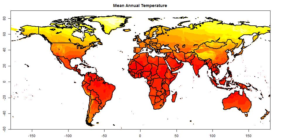
The raster layer of mean annual temperature can be downloaded here on the WorldClim website.
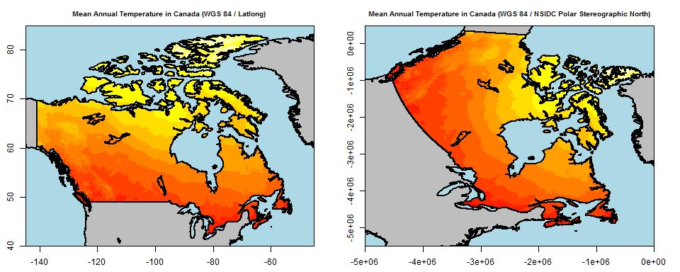
Example 3:
pol=SpacializedMap('worldHires','Canada',exact=F)
pol_rasterized=rasterize(pol,MAT)
pol_rasterized=crop(pol_rasterized,extent(c(-145,-45,40,85)))
MAT=crop(MAT,extent(c(-145,-45,40,85)))
values(MAT)[is.na(values(pol_rasterized))]=NA
X11(20,8)
par(mfrow=c(1,2),mar=rep(2.5,4))
image(matrix(1),xlim=c(-145,-45),ylim=c(40,85),col="lightblue",main="Mean Annual Temperature in Canada (WGS 84 / Latlong)",cex.main=.8)
image(MAT,add=T,col=rev(heat.colors(12)))
plot(SpacializedMap('worldHires','USA'),col="grey",add=T,lwd=2)
plot(SpacializedMap('worldHires','Greenland'),col="grey",add=T,lwd=2)
plot(SpacializedMap('worldHires','Canada'),add=T,lwd=2)
box()
MAT=projectRaster(MAT,crs=CRSargs(CRS("+init=epsg:3413")))
image(matrix(1),xlim=c(-5e+6,0),ylim=c(-5.5e+6,.5e+6),col="lightblue",main="Mean Annual Temperature in Canada (WGS 84 / NSIDC Polar Stereographic North)",cex.main=.8)
image(MAT,add=T,col=rev(heat.colors(12)))
plot(spTransform(SpacializedMap('worldHires','USA'),CRS("+init=epsg:3413")),col="grey",add=T,lwd=2)
plot(spTransform(SpacializedMap('worldHires','Greenland'),CRS("+init=epsg:3413")),col="grey",add=T,lwd=2)
plot(spTransform(SpacializedMap('worldHires','Canada'),CRS("+init=epsg:3413")),add=T,lwd=2)
box()